Maximizing GPU Efficiency: The Battle of Inference Methods
From Triton Inference Server to PyTorch Batch Inference: How Batch Processing Delivers a 500% Speed Increase
Introduction

In the era of rapid advancements in deep learning, encompassing Large Language Models (LLMs), Vision Language Models (VLMs), Natural Language Processing (NLP), and Computer Vision (CV), companies are increasingly confronted with critical decisions regarding inference methodologies. The stakes are high, as choosing the wrong approach could potentially result in a fivefold increase or more in computational resources for the same workload.
Two primary strategies dominate the landscape of model deployment: online inference and batch inference. While numerous articles discuss these approaches in theory, there's a notable lack of comprehensive benchmarks comparing their performance. This article aims to fill that gap by presenting a data-driven analysis, offering concrete metrics to illustrate the significant differences between these two inference methods.
By examining hard numbers and performance metrics, we'll provide valuable insights to help organizations make informed decisions about their inference strategies, potentially saving substantial computational resources and optimizing their AI workflows.
Inference in Deep Learning
Once a model is trained, extracting meaningful results requires performing inference - the process of running a forward pass through the model to obtain outputs. Inference mode differs from training mode in several key aspects:
Gradient Computation: During inference, gradients are not necessary. Failing to disable gradient computation can lead to unnecessary computational overhead. In PyTorch, this is typically achieved using context managers such as
torch.no_grad()ortorch.inference_mode().Layer Behavior: Certain layers, such as batch normalization and dropout, behave differently during inference compared to training. To ensure consistent predictions, it's crucial to set the model to evaluation mode by calling
model.eval(). Forgetting this step can result in inconsistent model outputs.Performance Optimization: Inference mode often allows for various optimizations that can significantly improve speed and efficiency.
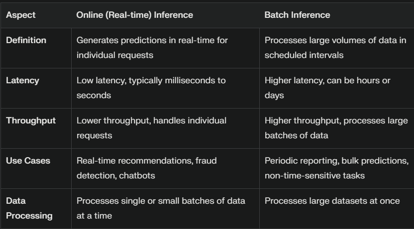
When considering inference strategies, two main paradigms emerge: batch inference and online inference. Each approach has its own set of characteristics and use cases, which we will explore in detail.
Batch Inference
Batch inference is a powerful technique for processing large volumes of data efficiently. This method involves performing inference on data in batches, leveraging highly optimized dataloaders for loading and preprocessing.
Key Characteristics
Bulk Data Processing: Ideal for scenarios where data is available in large quantities and real-time results are not required.
GPU Optimization: Maximizes the utilization of GPU hardware, ensuring cost-effective processing.
Predictable Performance: Offers consistent throughput based on machine specifications, facilitating easy scaling to meet processing time requirements.
Advantages
Reduced Network Overhead: Minimizes the impact of network latency by downloading and processing data in bulk.
Simplified Setup: Generally easier to configure compared to online inference systems.
Stable Load Handling: Eliminates the need to manage sudden spikes in user requests, as there is no real-time traffic.
Deployment Considerations
While batch inference deployment is less complex than online systems, it still requires attention to:
Data Partitioning: Determining optimal batch sizes for processing
Error Handling: Implementing robust error management strategies
Service Level Agreements (SLAs): Meeting agreed-upon deadlines for data processing and delivery
Batch inference provides a streamlined approach to large-scale data processing, offering efficiency and predictability for scenarios where real-time results are not critical.
Online Inference
Online inference, also known as real-time inference, is a sophisticated approach to processing incoming requests with minimal delay. This method is crucial for applications requiring immediate or near-immediate responses.
Key Features
Low Latency: The primary focus is on delivering results as quickly as possible, often within milliseconds.
Continuous Processing: Handles incoming requests in real-time, as opposed to processing data in batches.
Complex Engineering: Requires advanced techniques and optimizations to achieve high performance.
Applications and Challenges
Online inference is exemplified by chatbot-style deployments of Large Language Models (LLMs), where instant responses are essential. However, this approach presents significant challenges:
Technical Complexity: Implementing online inference systems is considerably more difficult than batch processing.
Optimization Efforts: Substantial research and engineering work is dedicated to enhancing performance through:
Development of optimized Triton kernels
Quantization techniques
Use of high-performance programming languages like Rust and C++
Considerations
Given the complexities involved, it's crucial to carefully evaluate whether your use case truly requires real-time responses. If immediate results are not essential, batch inference may be a more efficient and cost-effective alternative. Online inference represents the cutting edge of real-time data processing, offering immediate results at the cost of increased complexity and resource demands.
Benchmark Setup
The second half of the article will focus on benchmarking of batch vs online inference. We start with the benchmark setup by looking at the dataset, model, and the machine specs.
Dataset: For this experiment I’ll be using the mehdiiraqui/twitter_disaster dataset. It has 10,876 rows. We shall be processing the text column.
Model: I’ll be using the intfloat/multilingual-e5-base model for this evaluation. It is a encoder style model based on the xlm-roberta-base architecture.
Machine Specs: 13th Gen Intel(R) Core(TM) i9-13900HX, 32GB memory, RTX 4090 mobile.
Next, we look at the batch and online inference setup.
Batch Inference
For batch inference we will be using the vanilla pytorch dataloader. The batch_size is 32. We will be using inference_mode and bfloat16 for this evaluation. The main code for the inference is given below. We are not doing any optimization in terms of TensorRT export or compilation here.
    for input_batch in tqdm(dataloader):
        # Tokenization
        tokenization_start = time()
        tokenized_input = tokenizer(
            input_batch,
            truncation=True,
            padding=True,
            return_tensors="pt",
        ).to(device)
        tokenization_end = time()
        tokenization_time = (tokenization_end - tokenization_start) * 1000
        # Inference
        inference_start = time()
        with torch.inference_mode():
            with torch.autocast(device.type, torch.bfloat16) if device.type in [
                "cpu",
                "cuda",
            ] else nullcontext():
                output = model(**tokenized_input)
        inference_end = time()
        inference_time = (inference_end - inference_start) * 1000

        # Pooling
        pooling_start = time()
        if "pooler_output" in output.keys():
            embedding = output["pooler_output"]
        elif "last_hidden_state" in output.keys():
            embedding = output["last_hidden_state"][:, 0, :]
        else:
            raise ValueError(
                "Neither 'pooler_output' nor 'last_hidden_state' in model output."
            )
        embedding = embedding.detach().cpu().tolist()
        embedding_list.extend(embedding)
        pooling_end = time()
        pooling_time = (pooling_end - pooling_start) * 1000

        # Record batch profile
        batch_profiles.append([tokenization_time, inference_time, pooling_time])
Triton Inference Server
The triton inference server setup is pretty straightforward. We created pbtxt files and corresponding model files in the format triton inference server expects. We will be testing TensorRT and ONNX exports using different floating point precision. Explaining how to do ONNX and TensorRT export is left for another article. But the pbtxt config used for the TensorRT bf16 version is given below.
platform: "tensorrt_plan"
max_batch_size: 0
input [
  {
    name: "input_ids"
    data_type: TYPE_INT32
    dims: [ -1, -1 ]
  },
  {
    name: "attention_mask"
    data_type: TYPE_INT32
    dims: [ -1, -1 ]
  }
]
output [
  {
    name: "last_hidden_state"
    data_type: TYPE_FP32
    dims: [ -1, -1, 768 ]
  },
    {
    name: "cls_embedding"
    data_type: TYPE_FP32
    dims: [ -1, 768 ]
  }
]
We will do two types of server testing.
First is using perf_analyzer provided by Nvidia for all the different configurations.
Second is making API calls to the best performing version to profile batch inference.
The TensorRT export base command is:
trtexec --onnx=model.onnx --saveEngine=model.plan --useCudaGraph --minShapes=input_ids:1x1','attention_mask:1x1 --optShapes=input_ids:32x128,attention_mask:32x128 --maxShapes=input_ids:32x512,attention_mask:32x512 --verbose --shapes=input_ids:32x512,attention_mask:32x512
This command uses NVIDIA's TensorRT (trtexec) to optimize an ONNX model for inference:
--onnx=model.onnx: Specifies the input ONNX model file.--saveEngine=model.plan: Saves the optimized TensorRT engine as 'model.plan'.--useCudaGraph: Enables CUDA graph optimization for potentially faster execution.--minShapes,--optShapes,--maxShapes: Define the minimum, optimal, and maximum input shapes for dynamic shape support.--verbose: Enables detailed output for debugging.--shapes: Specifies the input shapes for profiling.
This command optimizes the model for various input sizes, with a focus on batch sizes up to 32 and sequence lengths up to 512, saving the result as a TensorRT engine file. In addition to these we passed --bf16 and --best flags provided by trtexec.
The perf_analyser command used is shown below:
perf_analyzer -m multilingual-e5-base-onnx --shape input_ids:32,512 --shape attention_mask:32,512 --concurrency-range 1:4 -i grpc -u localhost:8001Connect to a Triton Inference Server running on localhost:8001 using gRPC.
Test the performance of the 'multilingual-e5-base-onnx' model.
Use input shapes of [32, 512] for both 'input_ids' and 'attention_mask'. This will be the max shapes the model will encounter since 512 is the max token length of the model.
Measure performance at concurrency levels 1, 2, 3, and 4.
Results
We will look at the perf_analyser results first. This will set up stage for using the best performing configuration for the comparison against the batch inference. The results are summarized on the following table. The column names are mapped as follows: ONNX → ONNX fp32, base → TensorRT fp32, bf16 → TensorRT bf16, best —> TensorRT best, ONNX-Half → ONNX fp16.
Throughput Comparison (infer/sec)
Latency Comparison (usec)
Key Observations
ONNX-Half Performance:
The ONNX-Half model shows improved performance compared to the regular ONNX model, but still lags behind the TensorRT Base, BF16, and Best models.
It demonstrates better throughput and lower latency than the regular ONNX model across all concurrency levels.
Throughput Ranking:
BF16 > Best > Base > ONNX-Half > ONNX
The BF16 and Best models maintain their significant lead in throughput, especially at higher concurrency levels.
Latency Ranking:
Best ≈ BF16 < Base < ONNX-Half < ONNX
The ONNX-Half model shows lower latency compared to the regular ONNX model but higher latency than the other variants.
Scalability:
The ONNX-Half model shows limited scalability, similar to the regular ONNX model. Its performance improves only slightly as concurrency increases.
BF16 and Best models continue to demonstrate the best scalability among all variants.
Optimal Concurrency:
For the ONNX-Half model, peak performance is achieved at concurrency 3, similar to the BF16 and Best models.
However, the performance gain for ONNX-Half is much less pronounced compared to BF16 and Best models.
Half-Precision Impact:
The use of half-precision (FP16) in the ONNX-Half model provides a noticeable improvement over the regular ONNX model, likely due to reduced memory bandwidth requirements and potentially faster computation on supporting hardware.
Despite this improvement, it still doesn't match the performance of the non-ONNX variants (Base, BF16, Best).
In conclusion, while the multilingual-e5-base-onnx-half model shows improved performance over the regular ONNX model, it still falls short of the Base, BF16, and Best variants in terms of both throughput and latency. The BF16 and Best models remain the top performers, offering significantly better performance across all concurrency levels. This test is done on the same machine, depending on your client and server the numbers can be higher.
Now since we have a winner configuration in terms of online inference performance, for the next part we will be comparing the TensorRT bfloat16 Triton Inference Server performance against batch inference. The server is tested by making API calls to it.
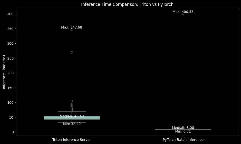
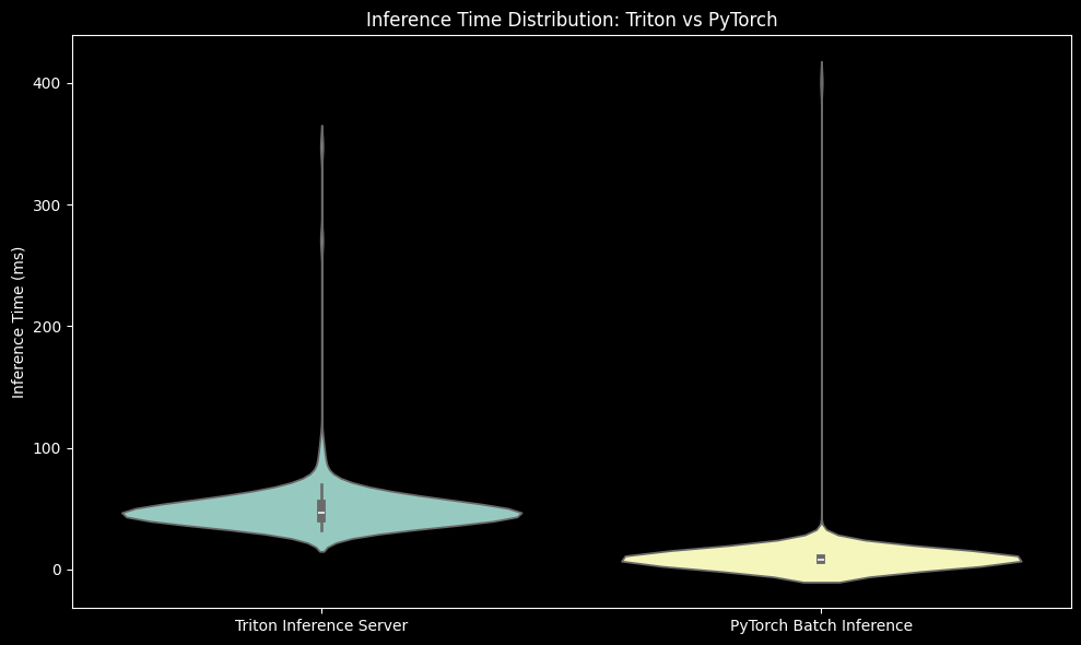
We record the inference time in milliseconds for all the batches. The comparison plots are shown below.
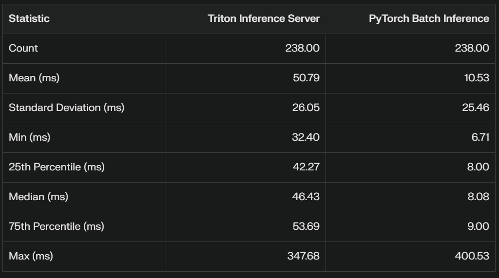
First is the boxplot, followed by violin plot and summary statistics for both the inference data.
This statistical summary provides valuable insights into the performance comparison between Triton Inference Server and PyTorch Batch Inference. Let's break down the key points:
Mean Inference Time:
Triton: 50.79 ms
PyTorch: 10.53 ms
PyTorch Batch Inference is significantly faster on average, with a mean inference time about 5 times lower than Triton.
Median (50th percentile):
Triton: 46.43 ms
PyTorch: 8.08 ms
The median values confirm that PyTorch is consistently faster, not just on average.
Variability (Standard Deviation):
Triton: 26.05 ms
PyTorch: 25.46 ms
Both methods have similar variability in inference times, indicating comparable consistency.
Range:
Triton: Min 32.40 ms, Max 347.68 ms
PyTorch: Min 6.71 ms, Max 400.53 ms
PyTorch has a lower minimum time but a slightly higher maximum time, suggesting it's generally faster but may have occasional outliers.
Interquartile Range (IQR):
Triton: 75% (53.69 ms) - 25% (42.27 ms) = 11.42 ms
PyTorch: 75% (9.00 ms) - 25% (8.00 ms) = 1.00 ms
PyTorch has a much smaller IQR, indicating more consistent performance across most runs.
Statistical Significance:
t-statistic: 17.05
p-value: 3.43e-51
The extremely low p-value (much less than 0.05) indicates that the difference in performance between Triton and PyTorch is statistically significant.
Conclusion
In this article, we looked at the two major ways for performing inference in deep learning namely batch inference and online inference. We looked at the pros and cons of each. We then conducted comprehensive benchmarking and analysis to reveal significant insights into the performance of online vs batch inference.
While Triton Inference Server with TensorRT optimization offers impressive scalability and throughput, especially in multi-client scenarios, PyTorch batch inference demonstrates superior performance in terms of raw inference speed for the appropriate use case.
PyTorch Batch Inference consistently outperformed Triton, with mean inference times approximately 5 times faster.
This stark difference highlights the importance of choosing the right inference method based on your specific requirements.
For applications that prioritize low-latency processing of large datasets in controlled environments, PyTorch batch inference is the clear winner.
However, it is crucial to note that Triton Inference Server still has its merits, particularly in scenarios involving multiple concurrent clients or when deployment flexibility and scalability are paramount.
The TensorRT optimizations, especially with BF16 precision, showed significant improvements over standard ONNX models.
Ultimately, the choice between online inference and batch Inference depends on your specific use case, infrastructure, and performance requirements. This benchmarking exercise underscores the importance of thorough testing and comparison when selecting an inference method for your deep learning models.
Making the wrong choice of selecting online inference if you clearly have a batch processing use case can cost you 5 times more money just in terms of compute cost. This doesn’t factor in the deployment complexity which can increase the total cost even more.


